
Why did the B2B sales win rate fall?
When a team wins fewer deals, did it close fewer opportunities, did the portfolio change, or did the same products win less often? This study separates those movements in a public CRM dataset.
1,000 credits + 7 days full accessOn first app sign-in · Once per device · No card required
We examined 6,064 opportunities that closed from April through December 2017 in a fictional B2B CRM archive. The win rate fell from 61.407% in Q3 to 60.252% in Q4. A symmetric decomposition gives +0.016 percentage points for product mix and −1.171 points for within-product rate changes. Of the 61 fewer wins, the lower volume of closures accounted for a larger component than the fall in win rate.
Win count and win rate answer different questions
A team sees fewer signed orders in its quarterly review. Before changing its pitch or pricing, it needs to know whether fewer deals reached a decision or whether the team won a smaller share of the deals that closed.
The number of wins counts opportunities marked won with a close date in the period. The closed-deal win rate divides that count by all wins and losses with a close date in the same period. Deals still open are outside the denominator. Order value and units sold are separate measures.
We first ask how much of the Q3-to-Q4 change in wins is associated with closure volume and how much is associated with the win rate. We then ask how much of the rate difference reflects a change in the product distribution versus changes in win rates within each product. We check an adjacent quarter pair, an alternate regional grouping and the effect of excluding one low-volume product.
A close-date rate describes the opportunities that reached an outcome in a reporting period. An entry cohort starts with opportunities opened in a given period and gives each one a defined follow-up window. The B2B sales forecast backtest addresses the probability of winning within a fixed horizon for deals open at a forecast date.
Define the reporting period and opportunity grain
Maven Analytics distributes CRM Sales Opportunities as sample data from a fictional computer hardware company. The pipeline table records an opportunity ID, a product, the final status and a close date where available.
| Population | Records | Treatment |
|---|---|---|
| Source opportunity table | 8,800 | All opportunity IDs are unique. |
| Open or prospecting | 2,089 | Outside the denominator for closed-deal win rate. |
| Closed outside the study period | 647 | Q1 recorded closures begin in March. We use the following three full calendar quarters. |
| Closed April to December 2017 | 6,064 | The three-quarter analysis covers seven products. |
We assign each deal to a calendar quarter by close date. Separate deals for the same customer remain separate opportunities. We use the product label as recorded in the pipeline file. For example, the archive spells GTXPro without a space. The main analysis does not require a product catalogue join.
For the sensitivity check, we match each salesperson to the region in the sales team file. The lookup has unique salesperson entries, and every included deal has a match. The archive contains no dated history of sales territory assignments. We use the region as reported in the export.
The analysis weights each opportunity equally. We did not weight by close_value. An amount-based version would require a comparable opportunity value for wins and losses, measured at an agreed point in the sales process.
Separate the change in deal volume from the change in win rate
| Period | Won | Lost | Total closed | Win rate |
|---|---|---|---|---|
| 2017 Q2 | 1,254 | 778 | 2,032 | 61.713% |
| 2017 Q3 | 1,257 | 790 | 2,047 | 61.407% |
| 2017 Q4 | 1,196 | 789 | 1,985 | 60.252% |
From Q2 to Q3, the team won three more deals while its win rate fell by about 0.306 percentage points. Fifteen more deals closed. Counts and rates can travel in different directions because the rate also depends on the denominator.
From Q3 to Q4, 62 fewer opportunities closed and wins fell by 61. Wins equal closures multiplied by the win rate. To separate the difference symmetrically, we multiply the change in closures by the average of the two rates. We multiply the change in rate by the average of the two closure counts. The resulting components add to the observed change in wins.
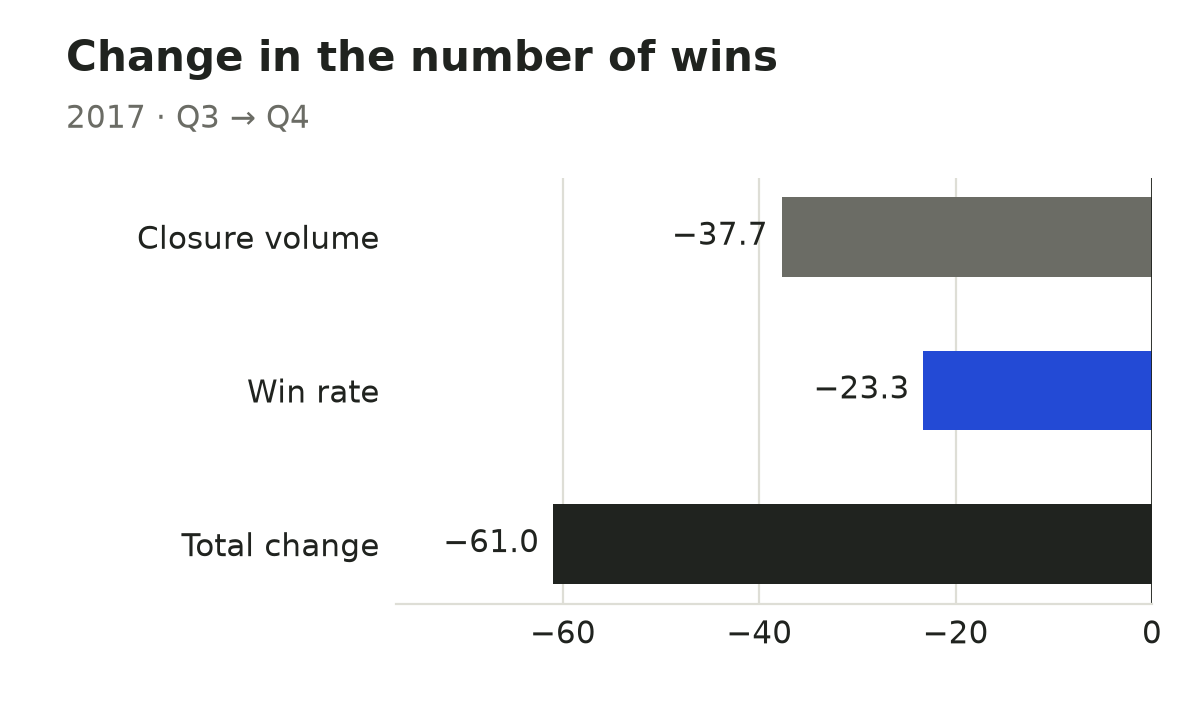
About −37.7 wins are associated with the closure volume component and −23.3 with the rate component. A lower closure volume is a prompt to check the number of new opportunities, the time to decision and which expected decisions slipped. Choosing among those explanations requires dated records of the open pipeline.
Separate product shares from win rates within each product
Each product has two measures. Its share is the fraction of all closed deals for that product. Its rate is the share of that product’s closed deals that were won. For example, if 20 of 100 closed opportunities involve one product and it wins 12 of those 20, its portfolio share is 20% and its win rate is 60%. Its contribution to the total rate is 20% × 60%, or 12 percentage points.
The aggregate rate equals the sum of those products of shares and rates. For the change between two dates, we use E. M. Kitagawa’s symmetric decomposition. Enter shares and rates as fractions. Multiply the resulting contribution by 100 to read it in percentage points.
| Component | Calculation for each product | What it measures |
|---|---|---|
| Mix | Change in product share × average product win rate across the two periods | Contribution associated with the distribution of closed deals across products. |
| Within-product rate | Change in product win rate × average product share across the two periods | Contribution associated with different win rates at a common product mix. |
| Total difference | Sum both contributions over all products | Exactly equals the difference between aggregate rates before rounding. |
The symmetric calculation uses both periods as the reference. Expand the two terms for any product and the cross-terms cancel. What remains is the later share multiplied by its rate, minus the earlier share multiplied by its rate. We use exact fractions in the code to check the identity before rounding published numbers.
A second way to inspect the within-product result is to calculate both rates using the same average product shares. On that reference distribution, the Q3 rate is 61.433% and the Q4 rate is 60.262%. The standardized difference is −1.171 points. The reference changes when we use a different pair of quarters. To create a comparable time series, hold the standard mix fixed across all its dates.
The net product mix contribution was close to zero
| Product | Q3 won / closed | Q4 won / closed | Mix | Within product |
|---|---|---|---|---|
| GTK 500 | 4 / 6 | 3 / 7 | +0.033 | −0.077 |
| GTX Basic | 256 / 419 | 257 / 411 | +0.146 | +0.295 |
| GTX Plus Basic | 212 / 330 | 178 / 328 | +0.239 | −1.628 |
| GTX Plus Pro | 143 / 234 | 143 / 227 | +0.003 | +0.215 |
| GTXPro | 226 / 368 | 200 / 325 | −0.987 | +0.022 |
| MG Advanced | 186 / 330 | 183 / 316 | −0.115 | +0.248 |
| MG Special | 230 / 360 | 232 / 371 | +0.698 | −0.246 |
| Total | 1,257 / 2,047 | 1,196 / 1,985 | +0.016 | −1.171 |
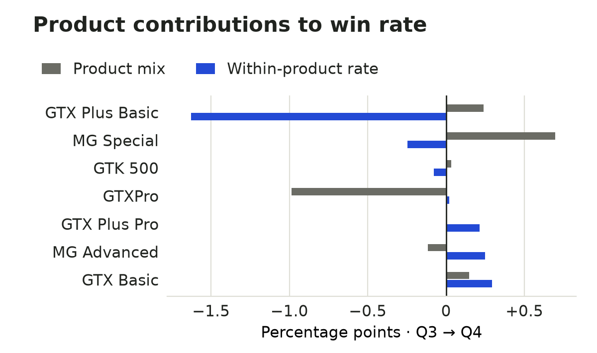
The mix component of +0.016 points combines larger changes with opposite signs. GTXPro’s share of closed deals decreased from 17.98% to 16.37%, for a mix component of −0.987 points. MG Special’s share rose from 17.59% to 18.69%, contributing +0.698 points. Showing only the net would hide how those movements offset one another.
For GTX Plus Basic, the number of closures changed from 330 to 328. Wins fell from 212 to 178 and the product win rate fell from 64.24% to 54.27%. The within-product component was −1.628 points. Positive contributions from other products offset part of that fall, so a single group’s contribution can exceed the magnitude of the overall change.
A useful follow-up is to pull comparable GTX Plus Basic deals from both quarters. Did buyers consider the product for the same jobs? Had the decision dates changed? Did more buyers choose a different configuration? The archive contains no offers or buyer explanations. Use recorded replies and comparable interviews to investigate a process decision. The sales win-loss analysis guide provides a way to structure that work.
Both products can improve while the aggregate rate falls
| Group | Earlier period | Later period | Rate difference |
|---|---|---|---|
| Product A | 64 / 80 · 80% | 17 / 20 · 85% | +5 percentage points |
| Product B | 4 / 20 · 20% | 20 / 80 · 25% | +5 percentage points |
| All deals | 68 / 100 · 68% | 37 / 100 · 37% | −31 percentage points |
Each product improved by five points. Product B, which had the lower win rate in both periods, accounted for 80% of the later portfolio. The total fell by 31 points. The symmetric identity gives −36 points for mix and +5 for changes within products. At a fixed 50/50 mix, the rate rises from 50% to 55%.
This constructed example shows the direction reversal associated with Simpson’s paradox. We created the numbers to illustrate the mechanism. In the CRM archive, some product rates improved and others declined. The example shows why checking the groups matters before drawing conclusions from the headline rate.
Repeat the comparison by region and without a sparse product
| Comparison | Total difference | Mix contribution | Within-group contribution |
|---|---|---|---|
| Product · Q2 → Q3 | −0.306 | +0.046 | −0.352 |
| Product · Q3 → Q4 | −1.155 | +0.016 | −1.171 |
| Region · Q3 → Q4 | −1.155 | +0.027 | −1.182 |
| Product excluding GTK 500 · Q3 → Q4 | −1.078 | +0.019 | −1.098 |
GTK 500 had six closed opportunities in Q3 and seven in Q4. One outcome can move the win rate for a group that small. Excluding it changes both the population and the win rate difference. The result still assigns most of the observed fall to within-product rate changes. Keep the denominators visible alongside those rates.
The region analysis gives a small net mix contribution as well. Product and region are two separate ways to group the same deals. Their contributions both reconcile to the same raw difference. Adding them would count the same change twice. To examine whether the pattern varies by combinations of product and region, create a separate joint grouping and show how many records support each cell.
The Q2-to-Q3 comparison has a smaller raw decline and the same signs for both components. The quarters still come from one synthetic archive. Replicating the arithmetic for adjacent periods does not support a general claim about firms or industries.
Bring counts and reconciled contributions to the next review
Set the denominator in advance.
Use one record per opportunity. Define the treatment of declined, cancelled and no-decision records. Apply the same status and close-date rules to both periods.
Put the raw counts on the first line.
Show wins, losses, all closures and the win rate side by side. State the period and the direction of the comparison.
Choose a grouping that matches the decision.
Use product to review changes in the offer and region to review territory outcomes. Keep group counts, shares and win rates for both periods.
Reconcile the contributions to the headline change.
Sum mix and within-group terms before rounding. The result should equal the difference between the two raw rates.
Read the underlying deals.
For a group that contributes materially to the change, check matched opportunities, the agreed scope and buyer feedback before changing the process.
A new product may have no closed opportunities in the earlier period. Its earlier win rate is undefined. Setting that rate to zero would assign an artificial difference to the within-product component. One option is to decompose the shared products and report new or discontinued products separately. Show both the common-population and full-portfolio rates.
For regular reporting, pick a reference product mix and keep it fixed across periods. Show the standardized rate alongside the actual rate. An operations team planning for the observed volume may care about the current mix. A team examining the same products across time may care about the standardized comparison.
The decomposition identifies where to investigate
The archive represents a fictional company, one year and a single product label per deal. The results describe recorded closures. The method cannot recover deals removed before export, deals reopened later or changes to earlier product assignments.
Within-product rate changes include shifts in customer type, sales process, review timing and any other factors that differ within a group. The exercise estimates no causal effects. To test a particular explanation, gather dated stage histories, the offers sent to comparable buyers and direct buyer feedback.
A close-date view can appear healthier when difficult deals remain open for longer. Examine a fixed-horizon entry cohort and the proportion still unresolved if this could matter for your reporting. Keep the definitions explicit when the two views appear together.
Opportunities may share customers and sales teams. We report descriptive results from a synthetic archive without confidence intervals or significance claims. The article is a technical study published with its method and aggregate outputs. It has undergone no external peer review.
Recreate the analysis from the original ZIP
The references link to the dataset publisher and a public archive mirror. Two public copies gave the same SHA-256 digest. The script checks that digest before running. Place the script and archive in the same directory and run python reproduce.py CRM+Sales+Opportunities.zip. Substitute the local file name if it differs.
Python 3.10 or later. The analysis uses the standard library.
Counts, shares, rates and contributions by dataset grouping and period. Shares, rates and signed contributions are stored as fractions.
Includes exclusions, quarterly totals, sensitivity comparisons and the archive fingerprint.
The figure script uses Matplotlib to plot the summary. We independently recomputed the main counts and both product terms with a SQLite query. The outputs matched.
Use the aggregate rate to decide which records to inspect
The win rate fell in this archive while the net product mix component was slightly positive. Changes within products accounted for the decline in the rate. The fall in the number of wins had a larger closure-volume component.
The useful sequence for a review is to count the closures, compute the share won, and locate the groups that contributed to the difference. Read the underlying opportunities before committing to a change. This connects the metric to decisions buyers made and leaves room to test competing explanations.
Frequently asked questions
Answers about the denominator and the decomposition.
How do you calculate the B2B sales win rate?
Divide closed-won opportunities by closed-won plus closed-lost opportunities, using the same close-date period for both counts.
Can the number of wins rise while the win rate falls?
Yes. If closed volume grows faster than the number of wins, the count can rise while the winning share falls.
What is a percentage point?
It measures the difference between two percentages. A change from 60% to 58% is a decline of two percentage points.
How can product mix change a sales win rate?
The aggregate rate is weighted by each product’s share of closures. If lower-win-rate products make up more of those closures, the aggregate can fall even when each product’s win rate stays the same.
What if a product has no earlier closures?
Report the decomposition for products present in both periods. Show the new product’s closures and wins separately.
Can these results serve as a benchmark for a sales team?
The dataset contains fictional opportunities. The article reports the method and the results obtained from that archive.
Sources and example notes
Sources for the data, measurement definition and decomposition method.
- Maven Analytics · CRM Sales Opportunities
The publisher describes the fictional sales dataset and its public domain licence.
- Public archive mirror · GitHub
Public copy of the archive used in the analysis.
- Salesforce Help · Calculate Win Rate on Closed Opportunities
Documents the closed-deal denominator and distinguishes it from all created opportunities.
- Kitagawa (1955) · Components of a Difference Between Two Rates
Introduces the decomposition of a rate difference into composition and within-group rate components.
- Michigan Department of Health and Human Services · Kitagawa rate decomposition
An applied public reference for the symmetric formulas.
- Simpson (1951) · The Interpretation of Interaction in Contingency Tables
Original scholarly context for studying combined and stratified associations.