
How to backtest B2B sales forecasts
What is the chance that an open deal will be won within 30 days? This study compares three estimates across 18 weekly CRM snapshots, with reproducible code and results.
1,000 credits + 7 days full accessOn first app sign-in · Once per device · No card required
Starting from 8,800 fictional CRM records, we scored 40,800 forecasts for 4,791 distinct opportunities across 18 weekly test dates. At 30 days, the historical closed-deal win rate had a Brier score of 0.3729. Matching the forecast horizon reduced the score to 0.1033. Adding deal age gave 0.1049 and improved the score at 60 days. The results show why the forecast horizon needs to be defined before comparing models.
Define the event a 30-day sales forecast should predict
Suppose an open deal shows 60% in the CRM on July 1. That number could describe the chance of winning eventually, closing this month or winning this month. Each interpretation leads to a different forecast.
The event in this study is a win during the next 30 calendar days for a deal that had entered engagement and remained open at the end of the forecast date. A deal lost during that window has an outcome of zero. A deal still open at the deadline also scores zero for that forecast, even if it wins on day 31.
We asked two questions. Does a historical rate defined for the forecast horizon score better than the share of wins among closed deals? Can the time since first engagement improve that horizon-matched baseline? We repeated the comparison at 15 and 60 days to see whether the choice of horizon changed the result.
IBM researchers have framed B2B win propensity as the probability of winning ongoing opportunities within a defined time window. Rezazadeh’s field study used a richer CRM feature set at a consulting company to predict sales outcomes. Our study uses an inspectable starting point based on open deals and their age. The references below identify the setting for each study.
Which opportunities can be placed in a historical snapshot?
Maven Analytics describes CRM Sales Opportunities as sample data from a fictional computer hardware company. Each row in the pipeline file represents an opportunity.
| Final status | Opportunities | Role in the study |
|---|---|---|
| Won | 4,238 | First engagement and close dates available. The win becomes known on the close date. |
| Lost | 2,473 | First engagement and close dates available. The deal can enter a forecast before it closes. |
| Engaging | 1,589 | First engagement date available. No closure recorded by the end of follow-up. |
| Prospecting | 500 | First engagement date missing. The record cannot be placed in a historical snapshot. |
| Total | 8,800 | All IDs are unique. The 8,300 records with an engagement date are eligible for reconstruction. |
The data dictionary defines engage_date as the start of the Engaging stage. close_date records when a deal was won or lost. All 6,711 closed records have dates in the expected order. Close dates run from March 1 to December 31, 2017. We started historical snapshots on March 6 and treated December 31 as the end of follow-up.
Two public mirrors returned a ZIP with the same SHA-256 hash. We used only the pipeline file. The analysis does not need joins to the products, accounts or sales team tables. The final deal_stage field determines the outcome when a closure date becomes observable. It is never an input feature for an open deal.
The export has no complete stage history. It gives no reliable way to see when someone backfilled a date, reopened a deal or changed the stage without closing it. Our reconstructed snapshots are approximations with a clear date rule. A CRM that stores timestamped snapshots or event history can test the same question with stronger evidence.
Freeze each forecast at the information available that day
For each Monday, we took an end-of-day snapshot. A deal enters if its engagement date is on or before that Monday and its close date is later or missing. A win counts if the close date falls after the forecast date and on or before the horizon deadline.
The test uses 18 Mondays from July 3 through October 30, 2017. Each week, we recalculate the model using historical snapshots only after their entire outcome windows have elapsed. For the July 3 forecast at 30 days, May 29 is the most recent eligible Monday. The June 5 snapshot reaches its 30-day deadline on July 5, so its results are unavailable on July 3.
| Fictional case | Eligible for the forecast? | 30-day outcome |
|---|---|---|
| Won on July 3 | No | Already closed when the forecast was made. |
| Open on July 3, won August 2 | Yes | 1. The last day of the window counts. |
| Open on July 3, won August 3 | Yes | 0. The win falls beyond the cutoff. |
| Open on July 3, lost July 12 | Yes | 0. No win within the window. |
| First engagement on July 4 | No | Outside the population at the forecast date. |
The same deal can appear in several weekly forecasts while it remains open. The primary analysis scores each opportunity and date pair. This reflects a manager reconsidering the same deal in successive meetings. In a sensitivity check, we score only the first test prediction for each distinct opportunity. We keep the original predictions for that subset.
The chronological split prevents results from a future snapshot from entering an earlier training window. A deal can still contribute historical evidence once its earlier window has matured. The overlap of deals and outcome windows makes observations dependent. We report differences across weeks and first appearances as descriptive checks.
Compare two horizon-matched models with a familiar CRM rate
| Estimator | Calculation at the forecast date | Target represented by the rate |
|---|---|---|
| Closed-deal win rate | Divide deals won to date by all deals won or lost to date. | Share of wins among closed opportunities. |
| Horizon baseline | Use every mature historical snapshot and calculate the share of its opportunity-date pairs won within the target horizon. | Pooled probability of a win within the horizon. |
| Age-specific horizon rate | Group the same mature observations into 0–29, 30–59, 60–89 and 90+ days. Estimate the horizon rate within each group. | Probability within the horizon conditional on the deal’s observed age group. |
Deal age is the time since first engagement. It can differ from the time spent continuously in the current stage. When an age group has fewer than 50 past observations, we substitute the horizon baseline for that group and week. The cutoff is a modelling choice. Its denominator is snapshot rows and can include a deal more than once.
The Brier score is the average of the squared differences between a probability and its observed outcome of 0 or 1. A forecast of 70% contributes 0.09 if the deal wins within the horizon and 0.49 if it does not. Lower is better. Every forecast row contributes the same weight regardless of deal size.
Calibration means that forecast probabilities agree with observed frequencies across repeated cases. A single probability of 20% can match the overall win frequency and still leave the sales team unable to distinguish deals. We therefore look at the Brier score alongside average forecast probabilities, observed rates and differences by deal age.
The closed-deal win rate overstated near-term wins
| Measure | Closed-deal win rate | Horizon baseline | Age-specific horizon rate |
|---|---|---|---|
| Mean forecast probability | 63.44% | 17.00% | 17.58% |
| Observed win frequency | 11.27% | 11.27% | 11.27% |
| Brier score | 0.37288 | 0.10333 | 0.10493 |
The test generated 40,800 forecasts for 4,791 distinct opportunities. There were 4,599 positive outcomes at 30 days. That count is tied to forecast rows. One win can create positive outcomes in more than one weekly snapshot.
The average closed-deal rate was 52.17 percentage points above the observed frequency. The horizon baseline reduced that gap to 5.73 points. Adding age increased the pooled Brier score by 0.00160 and the mean probability gap to 6.31 points. The horizon baseline scored best here, with room for better calibration.
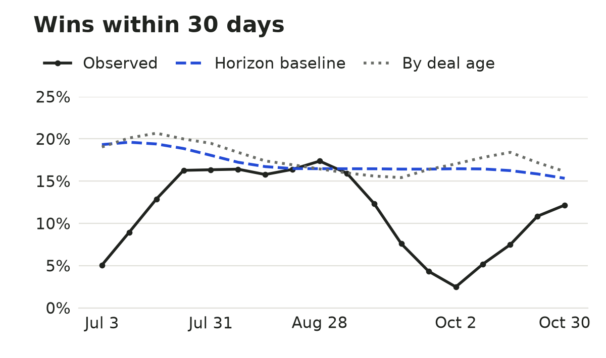
On July 3, 87 of 1,717 open deals won within 30 days. The observed rate was 5.1%, compared with 19.3% for the horizon baseline. By August 28 the observed rate was 17.4%, compared with 16.5% for the baseline. On October 2 it fell to 2.5%, with 61 wins from 2,452 eligible deals. The data cannot tell us whether that change reflects seasonality, the design of the synthetic data or a shift in the mix of opportunities.
Age groups showed different win rates and different forecast errors
| Days since engagement | Observations | Observed rate | Mean age-specific estimate |
|---|---|---|---|
| 0–29 | 11,106 | 10.97% | 11.08% |
| 30–59 | 9,844 | 12.18% | 14.86% |
| 60–89 | 7,492 | 21.16% | 31.38% |
| 90 or more | 12,358 | 4.83% | 17.23% |
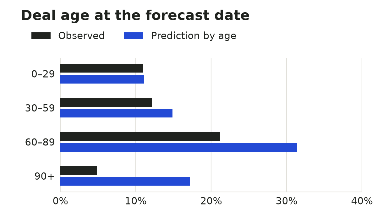
The 60–89-day group won most often within 30 days. The observed rate for the 90-day-and-over group was 12.40 percentage points below its estimate. The youngest group’s two averages were close. A rule that only makes the probability decline with each extra day would miss the higher observed rate in the middle of the age range in this export.
Age rates change with the weekly training set, so each bar averages many forecasts. Deal age can also be associated with opportunity characteristics missing from the export. This comparison identifies a difference in observed frequencies. It gives no estimate of the effect of making a buyer wait or of crossing a specific age boundary.
The preferred method changed with the forecast horizon
| Horizon | Observed win frequency | Horizon baseline | Age-specific rate | Weeks where age improved the score |
|---|---|---|---|---|
| 15 days | 6.31% | 0.06058 | 0.06158 | 9 of 18 |
| 30 days | 11.27% | 0.10333 | 0.10493 | 9 of 18 |
| 60 days | 21.31% | 0.17758 | 0.16784 | 17 of 18 |
At 60 days, age reduced the Brier score by 0.00974, about 5.5% relative to the horizon baseline. At 15 and 30 days it raised the pooled score. The 17 weeks at 60 days contain many of the same deals. This count describes how often the method yielded a lower score across the tested dates.
| Horizon | Distinct opportunities | Observed win frequency | Horizon baseline Brier | Age-specific Brier |
|---|---|---|---|---|
| 15 days | 4,791 | 13.55% | 0.11933 | 0.12275 |
| 30 days | 4,791 | 14.97% | 0.13001 | 0.13904 |
| 60 days | 4,791 | 24.84% | 0.19459 | 0.19227 |
Scoring each opportunity once retained the direction of the results. Adding age raised the score at 30 days and lowered it at 60 days. The first-appearance subset contains a different mix of deal ages and outcomes from the weekly portfolio. Compare the models within each table, where they share the same evaluation rows.
A 60-day historical outcome takes longer to become fully observable than a 30-day outcome. On a single forecast date, the two models can use different sets of mature history. Interpret the sensitivity results as a comparison across complete forecasting tasks, with both a different outcome and a different availability cutoff.
Design a test for your own sales process
Write one event and a deadline.
For example, define a win within 30 days for deals open at the end of Monday. Record which pipeline stages are eligible and how you handle same-day closures.
Store a dated copy of the information used for each forecast.
Keep the opportunity ID, forecast date, stage as known at the time, amount and currency, next action and expected decision date. Save actual closure and outcome as separate events.
Freeze a baseline and score both versions on the same dates.
Start with the historical rate for the target horizon. Add one candidate feature, such as stage or age, and compare on the same opportunities and time windows.
Measure probability and value separately.
Track observed win frequency and the Brier score. If you need expected order value, use the amount visible at the forecast date and score value errors separately.
Check the result prospectively.
If the model overpredicts, inspect forecast eligibility, dated decisions and data collection first. Run the same protocol on new forecasts before using the model in a decision.
Write down which decision the forecast feeds. Staffing for the next month may depend on the expected number or total value of jobs. Choosing which buyer to contact next may depend on rank within the pipeline. Evaluate the metric that matches the decision.
The weighted sales forecast guide shows how to calculate order estimates in a spreadsheet. The sales pipeline stages guide covers stage criteria. The models in this article run in the research code below.
What the results can support
The study uses one fictional data source and tests 18 dates in 2017. The rates apply to this archive and protocol. They provide no industry benchmarks and no evidence about outcomes for Anivo customers. This article is a technical study without external peer review.
The study population begins at first engagement. It omits 500 prospecting records without a date, so the results cannot speak to lead discovery or prior funnel steps. Opportunities still in Engaging at the end have no known eventual outcome in the archive.
The export provides no revisions to earlier entries and no comprehensive stage log. Within-day order is unknown. Retrospective edits or a deal reopened before the final export could change the reconstructed population. A production study should compare the reconstruction with archived snapshots and ingestion timestamps.
Repeated deals and overlapping test windows create dependence. We do not report confidence intervals or infer causal effects. Longer time coverage, more than one observed sales process and prospectively stored snapshots would help evaluate whether the same model ranking holds. We avoid using close_value, which is associated with the final outcome, to predict the future.
Recompute the tables from the source archive
The references identify the dataset publisher, licence and public mirror. The script checks the ZIP’s SHA-256 digest and stops on a mismatch. Use the original ZIP as the input. The site provides the code and aggregate outputs.
Requires Python 3.10 or later. The analysis uses only the standard library.
Place the script and archive in the same directory and run python reproduce.py CRM+Sales+Opportunities.zip. Substitute the filename if your archive has a different local name. The script writes the weekly data to CSV and the aggregate figures, date rules and archive fingerprint to JSON.
Contains the forecast date, horizon, counts, average probabilities and Brier scores for each week.
Includes data checks, pooled scores, age splits, first-observation results and the archive fingerprint.
The figure script reads the two outputs and draws the charts with Matplotlib. We independently checked the 30-day counts and Brier scores for both horizon-matched methods with a SQLite query.
Fix the event and timeline before changing the model
The largest error came from using a closed-deal win rate to estimate near-term wins in an open portfolio. Matching the historical event to the 30-day forecast gave a lower loss. Deal age helped at 60 days and raised the error at 30 days.
The practical conclusion is to archive what was known at each forecast date and evaluate what happened by a stated deadline. Add complexity only after scoring it against a horizon-matched baseline on the same out-of-sample forecasts.
Frequently asked questions
Definitions and scope of the forecast study.
How should I interpret a Brier score?
It is the mean squared difference between the probability and a 0 or 1 outcome. Lower is better when forecasts are scored on the same event, dates and observations.
Does the study use real customer records?
It uses fictional opportunities distributed by Maven Analytics. The reported results come from running the analysis on that archive.
Why does the closed-deal rate exceed the 30-day win frequency?
It conditions on deals that have closed. Its denominator leaves out open deals that may remain unresolved through the 30-day forecast window.
How did you treat a win after the deadline?
We kept the actual win and its date. For an earlier forecast whose deadline had passed, the outcome for that prediction was zero.
Does this model estimate revenue?
The model estimates a win within a chosen horizon. Estimating the value of expected orders also requires the amount known at forecast time and a separate value-based evaluation.
How would stage history change the test?
You could preserve the stage and time in stage at each forecast date. Test each candidate field against the same horizon baseline on the same snapshots.
Sources and example notes
Dataset, public mirror and methodological references.
- Maven Analytics · CRM Sales Opportunities
The publisher describes the archive as fictional and lists a public domain licence.
- Public archive mirror · GitHub
Mirror of the ZIP used in the analysis. Check its SHA-256 digest against the script.
- Yan et al. (2015) · Sales pipeline win propensity prediction
Defines a B2B win propensity task within a specific window for ongoing opportunities.
- Rezazadeh (2020) · A Generalized Flow for B2B Sales Predictive Modeling
Field study using a consulting firm’s CRM data and a richer feature set.
- Tashman (2000) · Out-of-sample tests of forecasting accuracy
Discusses rolling origins, model updates and out-of-sample forecast comparisons.
- Gneiting and Raftery (2007) · Strictly Proper Scoring Rules, Prediction, and Estimation
Discusses proper scoring rules and the theoretical basis for using Brier scores.